Thanks to Rod Trent at myITforum.com for pointing out this comparison (from Microsoft) of the various versions of Windows Mobile. The table has 61 rows of various features, and then shows which versions of Windows Mobile 5.0, 6.0, or 6.1 (with touch screen or without) have the feature.

I only recently learned that you get fewer features if your phone doesn’t have a touch screen! And I’m supposed to know it all.

Now I just need to find a comparison between Palm Activesync and what you get with Windows Mobile…

At the beginning of each year, I like to calculate the rate of return of each of my accounts for the previous year. If I haven’t added to or subtracted from an account, that’s as easy as (gain or loss) divided by initial investment. So, if I started with $10,000 and ended up with $12,000, my return was $2000 / $10000 = 0.20, or 20%.

But what if I added $1000 at some point during the year? Depending on when I added the $1000, it would be contributing various amounts to my return. This is where Excel’s XIRR function becomes very handy (other spreadsheets have it too). The XIRR function is used to determine the rate of return with irregular payments (IRR can be used if the payments are on a regular schedule).

I found a good explanation of calculating investment rate of return here, but really like Allen Wyatt’s ExcelTips article on the XIRR function. He explains how you use the function–really, you just need to remember that money put in the account is expressed as negative numbers, and money pulled out of the account (or remaining at the end) is a positive. You give the XIRR function the dates and amounts for the start, payments/withdrawals, and ending value, and it gives you a rate of return.

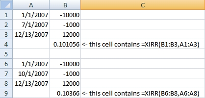
Notice in the following example how I started with $10,000, added $1000, and ended up with $12,000. Depending on when I added the $1000, the return varied from 10.1% to almost 10.4%.

Allen Wyatt has WordTips and ExcelTips that are searchable. Check out www.vitalnews.com.

I’ve bumped into this problem several times, and seem to forget the answer, so this is as much to remind me as for anyone else…

If you’re trying to manage the Windows XP firewall and the controls are grayed out, and you see the message “For your security, some settings are controlled by Group Policy”, the answer could be as simple as “you installed Windows Live OneCare”.

When you install Windows Live OneCare, it takes over the firewall settings.? To manually make changes, go to Start – Windows Live OneCare (or just click on the OneCare icon in the tray), then click the “Change settings” quick link.? From there you’ll have access to your firewall settings.

From NetworkWorld:? a list of the 20 most useful Microsoft sites for IT professionals.? You’ll probably find at least one useful site that you didn’t know about–I found several!